
Formatting the Data for TensorFlow
Part 1 of this blog series demonstrated the advantages of using a relational database to store and perform data exploration of images using simple SQL statements. In this tutorial, part 2, the data used in part one will be accessed from a MariaDB Server database and converted into the data structures needed by TensorFlow. The results of applying the model to classify new images will be stored in a relational table for further analysis.
This is a quick tutorial of a TensorFlow program with the details described as we go. If you are not familiar with the basic concepts, a good place to start is this TensorFlow tutorial, “Basic classification: Classify images of clothing“. Some of the examples and code in the tutorial are used here.
Additional Packages Needed
Some additional packages are needed for building and training the image classification model:
- Pickle implements binary protocols for serializing and de-serializing a Python object structure.
- NumPy provides support for large, multi-dimensional arrays and matrices, along with high-level mathematical functions to operate on these arrays.
- TensorFlow is a Python library for fast numerical computing. It is a foundation library that can be used to create Deep Learning models directly or by using wrapper libraries that simplify the process built on top of TensorFlow.
- Keras is an open-source neural-network library written in Python.
import pickle
import numpy as np
import tensorflow as tf

from tensorflow import keras
print('Tensorflow version: ', tf.__version__)
print('Numpy version: ', np.__version__)
Tensorflow version: 2.0.0
Numpy version: 1.16.2
Retrieve Images
Once the packages have been imported, the next step is to retrieve the training images from the database and split the data into two numpy arrays. First, we need to initialize the training images (train_images) and training labels (train_labels) arrays. Since we have already vectorized the images we can use the img_vector attribute to populate the train_images array with the SQL statement below.
# Initialize the numpy arrays
train_images = np.empty((60000,28,28), dtype='uint8')
train_labels = np.empty((60000), dtype='uint8')

# Retrieve the training images from the database
sql="SELECT img_label, img_vector, img_idx \
FROM tf_images INNER JOIN img_use ON img_use = use_id \
WHERE use_name = 'Training'"
cur.execute(sql)
result = cur.fetchall()

# Populate the numpy arrays. row[2] contains the image index
for row in result:
nparray = pickle.loads(row[1])
train_images[row[2]] = nparray
train_labels[row[2]] = row[0]
In a similar way, the images for testing can be retrieved from the database. The numpy arrays used in this case are test_images and test_labels. In this case, the testing data is 10,000 images at 28×28 pixel resolution.
# Initialize the numpy arrays
test_images = np.empty((10000,28,28), dtype='uint8')
test_labels = np.empty((10000), dtype='uint8')

# Retrieve the testing images from the database
sql="SELECT img_label, img_vector, img_idx \
FROM tf_images INNER JOIN img_use ON img_use = use_id \
WHERE use_name = 'Testing'"
cur.execute(sql)
result = cur.fetchall()

# Populate the numpy arrays. row[2] contains the image index
for row in result:
nparray = pickle.loads(row[1])
test_images[row[2]] = nparray
test_labels[row[2]] = row[0]
Finally, each image is mapped to a single label. The label names are stored in the categories table and loaded into the class_names array:
sql="SELECT class_name FROM categories"
cur.execute(sql)
class_names = cur.fetchall()
Preprocess the Data
The data must be preprocessed before training the network. If you inspect the first image in the training set, you will see that the pixel values fall in the range of 0 to 255:
plt.figure()
plt.imshow(train_images[0])
plt.colorbar()
plt.grid(False)
plt.show()
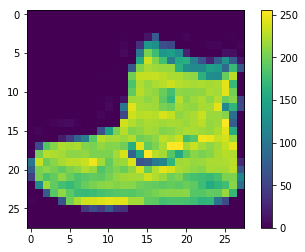
above: image from fashion_mnist dataset
Before feeding the images to the neural network model, the values need to be scaled to a range of 0 to 1. To do so, divide the values by 255. It’s important that the training set and the testing set are preprocessed in the same way.
You can use matplotlib to display the first 25 images to verify the data is in the correct format and ready for building and training the network:
train_images = train_images / 255.0
test_images = test_images / 255.0

plt.figure(figsize=(10,10))
for i in range(25):
plt.subplot(5,5,i+1)
plt.xticks([])
plt.yticks([])
plt.grid(False)
plt.imshow(train_images[i], cmap=plt.cm.binary)
plt.xlabel(class_names[train_labels[i]])
plt.show()
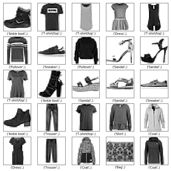
above: images from fashion_mnist dataset
Building the model
After the data has been preprocessed into two subsets, you can proceed with a model training. This process entails “feeding” the algorithm with training data. The algorithm will process the data and output a model that is able to find a target value (attribute) in new data — that is, classifying the image presented to the neural network.
Most deep learning neural networks are produced by chaining together simple layers.
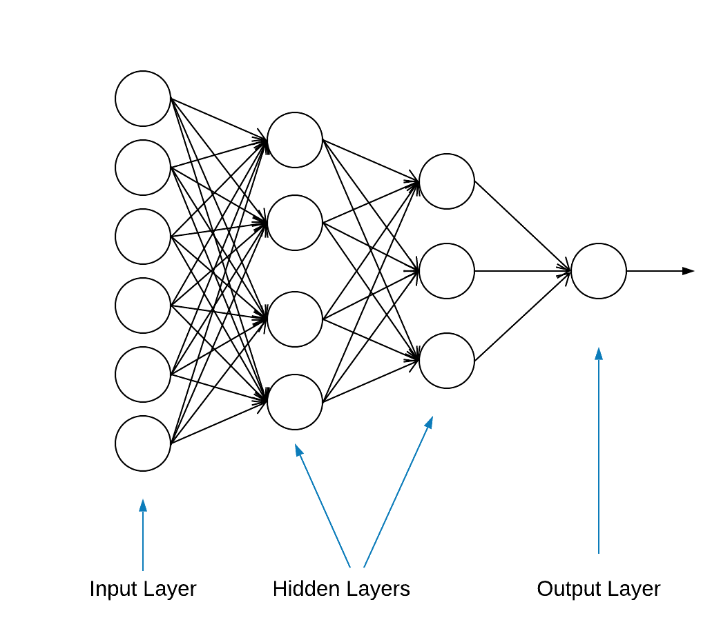
The first layer in the network transforms the image format from a two-dimensional array (of 28 by 28 pixels) to a one-dimensional array (of 28 * 28 = 784 pixels). This layer has no parameters to learn; it only reformats the data.
After the pixels are flattened, the network consists of two fully connected layers that need to be activated. In a neural network, the activation function is responsible for transforming the summed weighted input from the node into the activation of the node or output for that input.
The first dense layer has 128 nodes (or neurons) and is using a Rectified Linear Unit (ReLU) activation method. The rectified linear activation function is a piecewise linear function that will output the input directly if it is positive, otherwise, it will output zero.
The second (and last) layer is a 10-node softmax layer. A softmax function outputs a vector that represents the probability distributions of a list of potential outcomes. It returns an array of 10 probability scores that sum to 1. Each node contains a score that indicates the probability that the current image belongs to one of the 10 classes.
Most layers, such as tf.keras.layers.Dense, have parameters that are learned during training.
model = keras.Sequential([
keras.layers.Flatten(input_shape=(28, 28)),
keras.layers.Dense(128, activation='relu'),
keras.layers.Dense(10, activation='softmax')
])
Compiling the model
The model compilation step is used to add a few more settings before it is ready for training. In this case, the following settings are enabled.
- Optimizer—Updates the model based on the data it sees and its loss function (see below).
- Loss function—Measures how accurate the model is during training. You want to minimize this function to “steer” the model in the right direction.
- Metrics—Monitor the training and testing steps. The following example uses accuracy, the fraction of the images that are correctly classified.
model.compile(optimizer='adam',
loss='sparse_categorical_crossentropy',
metrics=['accuracy'])
Training the model
Training the neural network model requires the following steps.
- Feed the training data to the model.
- The model learns to associate images and labels.
- Make predictions about a test set.
- Verify that the predictions match the labels from the test_labels array.
To start training, call the model.fit method—so called because it “fits” the model to the training data:
model.fit(train_images, train_labels, epochs=10)
Train on 60000 samples
Epoch 1/10
60000/60000 [==============================] - 5s 83us/sample - loss: 0.4964 - accuracy: 0.8236
Epoch 2/10
60000/60000 [==============================] - 4s 65us/sample - loss: 0.3735 - accuracy: 0.8642
Epoch 3/10
60000/60000 [==============================] - 3s 55us/sample - loss: 0.3347 - accuracy: 0.8773
Epoch 4/10
60000/60000 [==============================] - 3s 56us/sample - loss: 0.3106 - accuracy: 0.8861
Epoch 5/10
60000/60000 [==============================] - 3s 58us/sample - loss: 0.2921 - accuracy: 0.8924s - loss: 0.2928 - accura - ETA: 0s - loss: 0.2925 - accuracy
Epoch 6/10
60000/60000 [==============================] - 3s 57us/sample - loss: 0.2796 - accuracy: 0.8969s
Epoch 7/10
60000/60000 [==============================] - 4s 70us/sample - loss: 0.2659 - accuracy: 0.9007
Epoch 8/10
60000/60000 [==============================] - 4s 61us/sample - loss: 0.2548 - accuracy: 0.9042
Epoch 9/10
60000/60000 [==============================] - 4s 61us/sample - loss: 0.2449 - accuracy: 0.9084
Epoch 10/10
60000/60000 [==============================] - 5s 76us/sample - loss: 0.2358 - accuracy: 0.9118
At the end of each epoch, the neural network is evaluated against the validation set. This is what loss and accuracy refer to.
Evaluate accuracy and predict
To estimate the overall accuracy of the model, calculate the average of all ten occurrences of the accuracy value, in this case 88%.
Then execute model.evaluate on the test set to get the predictive accuracy of the trained neural network on previously unseen data.
test_loss, test_acc = model.evaluate(test_images, test_labels, verbose=2)
10000/1 - 0s - loss: 0.2766 - accuracy: 0.8740
The test dataset is less accurate than the training dataset. In this case, this gap between training accuracy and test accuracy represents overfitting. The opposite is underfitting. If you want to learn more about this topic, I recommend Overfitting vs. Underfitting: A Conceptual Explanation by Will Koehrsen.
At this point, we can make some predictions about the images in our training data set.
predictions = model.predict(test_images)
predictions[0]
array([1.90860412e-08, 8.05085235e-11, 1.56402713e-08, 1.66699390e-10,
7.86950158e-11, 4.33062996e-06, 2.49049066e-08, 1.20656565e-02,
3.80084719e-09, 9.87929940e-01], dtype=float32)
The output of model.predict is an array of 10 numbers with the probability of an instance belonging to each class. Persisting the results in the MariaDB database for further analysis and reporting is a good idea. Below is an example of how to iterate on the predictions array to build a tuple and then insert it in the prediction_results table.
sql = "INSERT INTO prediction_results (
img_idx
, img_use
, T_shirt_Top
, Trouser
, Pullover
, Dress
, Coat
, Sandal
, Shirt
, Sneaker
, Bag
, Ankle_boot
, label)
VALUES (%s, %s, %s, %s, %s, %s, %s, %s, %s, %s, %s, %s, %s);"
i = 0
for row in predictions:
insert_tuple = (str(i), str(2)
, str(row[0]), str(row[1]), str(row[2]), str(row[3]), str(row[4])
, str(row[5]), str(row[6]), str(row[7]), str(row[8]), str(row[9])
, str(test_labels[i]))
cur.execute(sql, insert_tuple)
conn.commit()
i += 1
Once again, a simple SQL statement can be used to verify the data has been loaded.
sql = "SELECT T_shirt_Top
, Trouser
, Pullover
, Dress
, Coat
, Sandal
, Shirt
, Sneaker
, Bag
, Ankle_boot
, class_name as 'Test Label'
FROM prediction_results JOIN categories ON label = class_idx WHERE img_idx = 1"
display( pd.read_sql(sql,conn) )
| T_shirt_Top | Trouser | Pullover | Dress | Coat | Sandal | Shirt | Sneaker | Bag | Ankle_boot | Test Label |
| 0.00001 | 0.0 | 0.997912 | 0.0 | 0.001267 | 0.0 | 0.00081 | 0.0 | 0.0 | 0.0 | Pullover |
Plotting Predictions
A couple of plotting functions to display the predictions are defined below (Graphing functions).
Let’s retrieve a new image from the testing set and display the neural net classification based on the prediction probability.
sql = "SELECT img_idx, label FROM prediction_results WHERE img_idx = 1"
cur.execute(sql)
result = cur.fetchone()
plt.figure(figsize=(6,3))
plt.subplot(1,2,1)
plot_image(result[0], predictions[result[0]], test_labels, test_images)
plt.subplot(1,2,2)
plot_value_array(result[0], predictions[result[0]], test_labels)
plt.show()
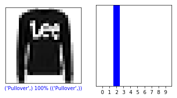
above: image from fashion_mnist dataset
In this case, the model was able to classify the image correctly with 100% accuracy. Next let’s execute a query to retrieve the first 15 images from the testing set and classify them.
sql = "SELECT img_idx, label FROM prediction_results LIMIT 15"
num_rows = 5
num_cols = 3
plt.figure(figsize=(2*2*num_cols, 2*num_rows))
cur.execute(sql)
result = cur.fetchall()
for row in result:
plt.subplot(num_rows, 2*num_cols, 2*row[0]+1)
plot_image(row[0], predictions[row[0]], test_labels, test_images)
plt.subplot(num_rows, 2*num_cols, 2*row[0]+2)
plot_value_array(row[0], predictions[row[0]], test_labels)
plt.tight_layout()
plt.show()
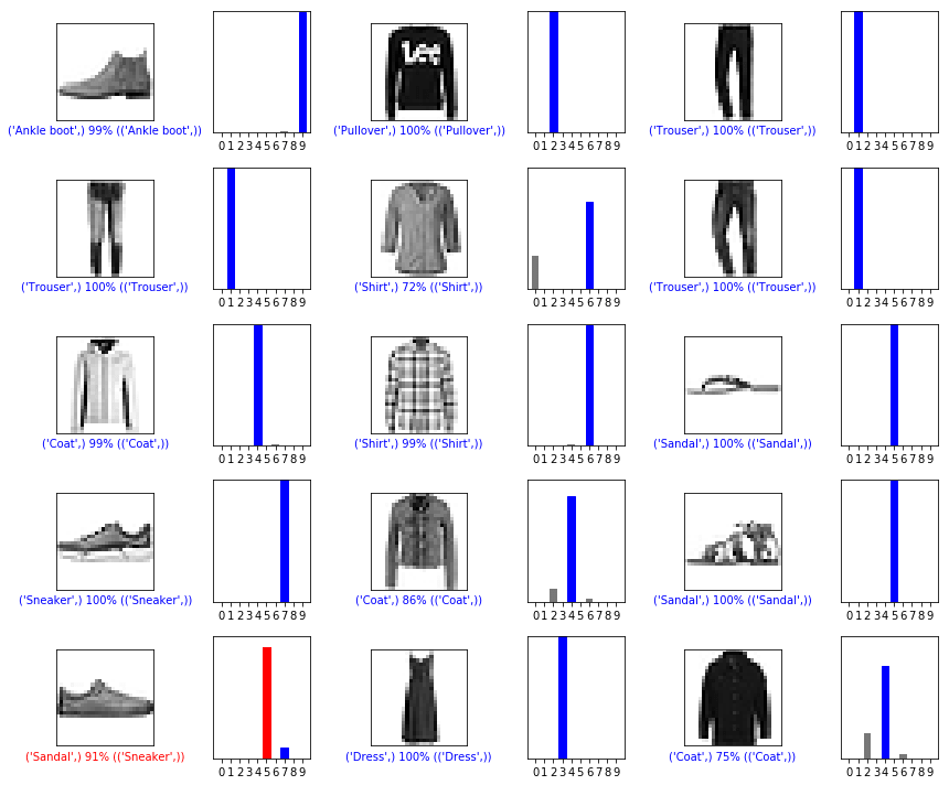
above: images from fashion_mnist dataset
As you can see, there will be instances where the model can be wrong as shown in the last row, left column. In this case, a sneaker was classified as a sandal (in red).
In Summary
Though integration between TensorFlow and MariaDB Server is easy, the benefits from this integration are substantial:
- Use of relational data within machine learning can reduce implementation complexity. Data Scientists and Data Engineers alike can use a common language to perform data wrangling and exploration tasks.
- Efficiency gained when accessing, updating, inserting, manipulating and modifying data can accelerate time-to-market.
- The ability to store the results of the model back to the database allows end-users and analysts to execute queries and reports using friendly reporting tools like Tableau.
MIT License
The Fashion MNIST (fashion_mnist) dataset leveraged by this blog is licensed under the MIT License, Copyright © 2017 Zalando SE, https://tech.zalando.com
The source code leveraged by this blog is adapted from the “Basic classification: Classify images of clothing” tutorial which is licensed under the MIT License, Copyright (c) 2017 François Chollet.
Permission is hereby granted, free of charge, to any person obtaining a copy of this software and associated documentation files (the “Software”), to deal in the Software without restriction, including without limitation the rights to use, copy, modify, merge, publish, distribute, sublicense, and/or sell copies of the Software, and to permit persons to whom the Software is furnished to do so, subject to the following conditions:
The above copyright notice and this permission notice shall be included in all copies or substantial portions of the Software.
THE SOFTWARE IS PROVIDED “AS IS”, WITHOUT WARRANTY OF ANY KIND, EXPRESS OR IMPLIED, INCLUDING BUT NOT LIMITED TO THE WARRANTIES OF MERCHANTABILITY, FITNESS FOR A PARTICULAR PURPOSE AND NONINFRINGEMENT. IN NO EVENT SHALL THE AUTHORS OR COPYRIGHT HOLDERS BE LIABLE FOR ANY CLAIM, DAMAGES OR OTHER LIABILITY, WHETHER IN AN ACTION OF CONTRACT, TORT OR OTHERWISE, ARISING FROM, OUT OF OR IN CONNECTION WITH THE SOFTWARE OR THE USE OR OTHER DEALINGS IN THE SOFTWARE.
References
Convert own image to MNIST’s image
matplotlib: Image tutorial
5 ways AI is transforming customer experience
Digitalization is reinventing business
What is image classification?
Introduction to the Python Deep Learning Library TensorFlow
Graphing functions
def plot_image(i, predictions_array, true_label, img):
predictions_array, true_label, img = predictions_array, true_label[i], img[i]
plt.grid(False)
plt.xticks([])
plt.yticks([])

plt.imshow(img, cmap=plt.cm.binary)

predicted_label = np.argmax(predictions_array)
if predicted_label == true_label:
color = 'blue'
else:
color = 'red'

plt.xlabel("{} {:2.0f}% ({})".format(class_names[predicted_label],
100*np.max(predictions_array),
class_names[true_label]),
color=color)

def plot_value_array(i, predictions_array, true_label):
predictions_array, true_label = predictions_array, true_label[i]
plt.grid(False)
plt.xticks(range(10))
plt.yticks([])
thisplot = plt.bar(range(10), predictions_array, color="#777777")
plt.ylim([0, 1])
predicted_label = np.argmax(predictions_array)

thisplot[predicted_label].set_color('red')
thisplot[true_label].set_color('blue')