Sometimes it’s the little things that matter.
While I have been (rightly) accused of routinely talking about open source strip mining by Amazon, or the failure of ERP by Oracle, and SAP causing the second coming of databases, you hardly ever hear me talk about Layer Trees and Bloom Filters as the future battleground in the cloud.
You’re probably thinking one of two things: either, it’s about time I talk about something substantial or why on earth would I spend any time on this? Bear with me.
Amazon AWS hosts more than 15 databases, some serverless, some relational, some document-based, some – yes – strip mined. Microsoft, Google and Alibaba offer fewer, but still many. Oracle, interestingly enough, presents itself as a single database – like MariaDB – but doesn’t quite know what to say about Berkeley DB, MySQL or TimesTen. Some applaud these vendors (give or take) in that they deem them “open.” In fact some usurp the word “open” and equate it with the concept of a supermarket with a blind eye on “house brands” taking the best shelf space.
We seem to have all this power at our fingertips. I believe it is all a façade. A misdirect, a giant snowball affecting the ability to expertly execute one’s use of technology and all the while degrading the goal of making technology work better. We use euphemisms like “eventual,” “glue,” “streaming,” “ETL,” “middleware,” even “best of breed” as misdirects and masks.
I believe the cloud, with these euphemisms, will have to change because I see big problems happening right now, stemming from pure neglect of the most important underlying element in the cloud: the data structure. What I see as the band-aid focus on using application-layer technologies to remedy this, causes invisible and visible shortcomings. Today’s modern applications depend on data that is consistent and truthful, and that’s not what we are getting today.

What the…!?! When you enter a new address or sales forecast into a database and it doesn’t show up when you run the report, you want to eat a pencil. Photo by JESHOOTS.COM on Unsplash.
I wrote this blog to help explain the most elemental parts of our database technology to better understand how we’re building a better cloud for all.
Part 1: Data Structures and Layer Trees
Intro to Data Structures
Let’s first define the phrase “data structure.” A comma delimited file is a data structure where each piece of independent data is followed by a comma. Those of you who use Excel have heard of a CSV file, which stands for comma-separated file. This type of data structure is rather dumb, forcing the person or program to know a lot about it, and is especially difficult when looking for something specific (if it is a large file). At times it can also take overnight for a complex spreadsheet to be refreshed, let alone using pivot tables. This type of file or data structure doesn’t offer ways to do things faster: it is flat, has a set of rows and columns, and has no data organization techniques to make data more searchable, unlike, in the extreme, a structure that we call a Layer Tree.
If you have heard of a Log-Structured Merge Tree (LSM), a Layer Tree is somewhat similar, or as one expert wrote, “it’s of the ‘discount bin knockoff variety.’” A LSM is a data structure “with performance characteristics that make it attractive for providing indexed access to files with high-insert volume.” Beyond the notion of indexes, which are used to locate data quickly – something that CSV files don’t have – an LSM data structure is most often associated with logs and key-value stores. In the MariaDB world, the MyRocks storage engine is based on RocksDB which is based on an LSM data structure. LSM data structures are wonderful for inserts and append-only applications, but not wonderful for “updating in place” a piece of data (such as current address), or fast reads (for analytical purposes) because it doesn’t innately reorganize data for complex queries (i.e., fragmented disk).
The key aspect of LSM that I want to focus on is the abstract concept of a “Tree.” In computer science, a Tree is used to break up large files of data into smaller files, such that it is faster to find a specific piece of data and perhaps change it (update or delete it). Computer science people sometimes refer to the left and right side of the tree; they also refer to a branch – connected to the main body of the tree – as nodes, with leafs (or children).
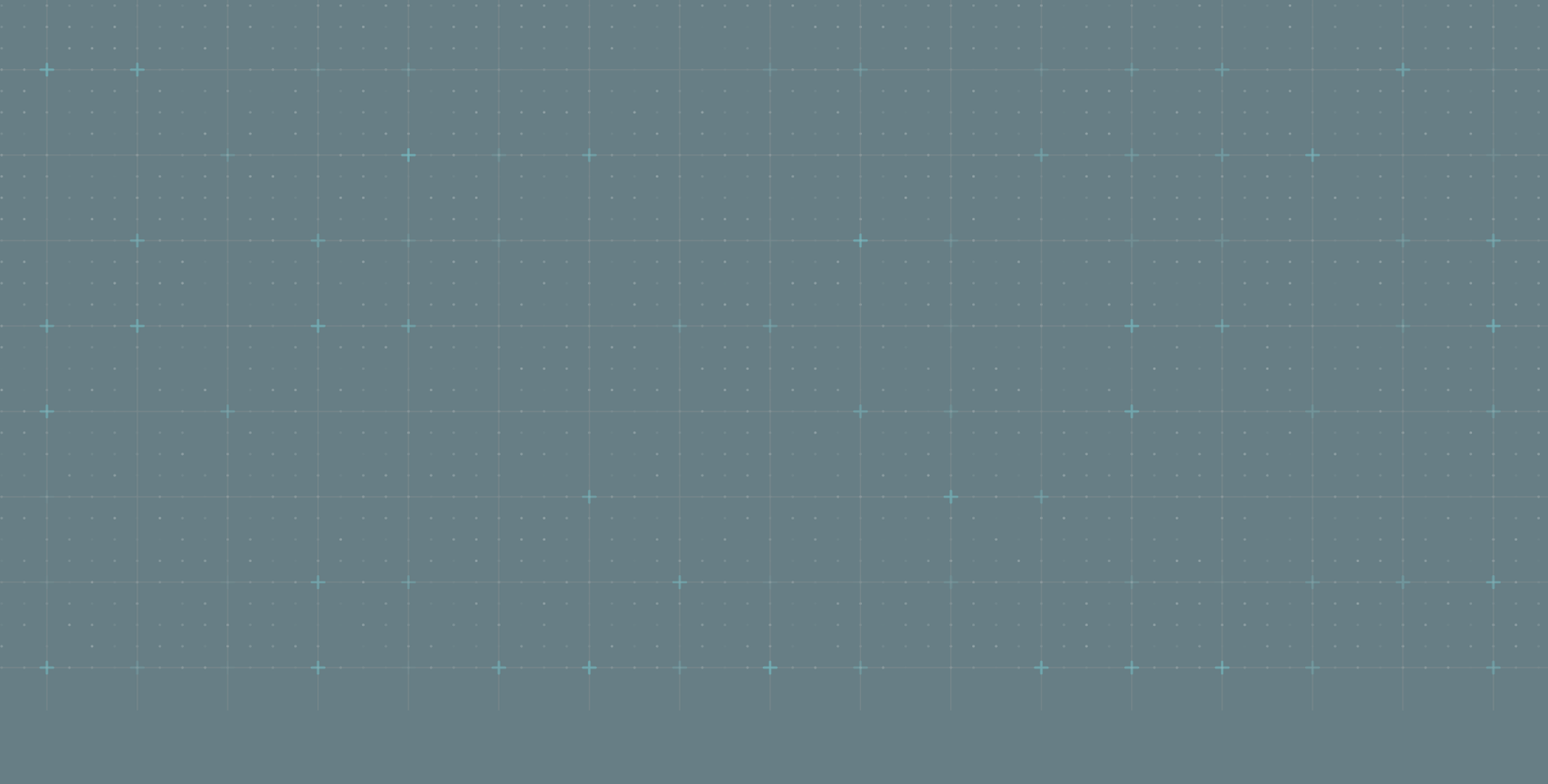
Think of a hierarchy of a company, from the CEO down. On one side of the company you might have the development organization (say the left side). On the right, you have the sales organization. Therefore, the development organization is a branch, as is sales. Below sales, you have different territories (which we could call nodes). Within each territory, there are sales people (called leafs or children). When you want to find a sales person in North America, your search steers you to the sales branch, then to the North American territory (node), and finally to the specific sales person you are looking for (leaf).
A development and sales hierarchy tree
A few years back, we acquired ClustrixDB, which uses a Layer Tree to improve write-heavy workloads. And as mentioned earlier, a Layer Tree is a variant of a LSM Tree; more specifically, a Layer Tree is a B-Tree with one or more additional B-Trees that serve as delta stores (ClustrixDB occasionally creates new delta stores to keep each individual delta store relatively small).
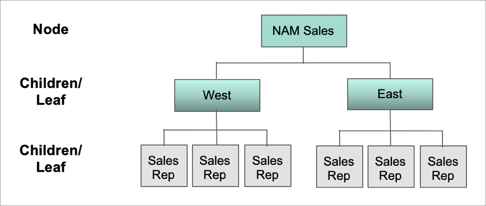
The Layer Tree
To understand a Layer Tree, we need to define a B-Tree. The “B” in B-Tree stands for balancing. Some think it stands for binary, for unknown reasons. What’s important here is not so much the details of data structures inside each layer – it is the very fact of being “layered.” They are like multi-storied buildings (pyramidal shape, with the square footage decreasing on the way up the stairs, and the main entrance located on the rooftop), plus well-designed pathways for inter-floor movements (merges), and hence clean and rapid methods of locating search targets on whichever floor they happened to be at any given time, while not in any way inhibiting the speed of their movements.
As for the interiors of the floors, and the features of the elevators and connecting stairs, the freedom of an architect’s creativity is infinite, and the evolution of best practices is steady and ongoing. There are implementations which do not use trees at all – memtables, skip lists, columnar containers, etc. I will leave this to others to argue which ones are “the best.”
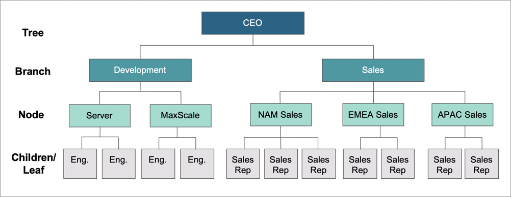
In the prior company hierarchy example, focusing on the sales side of the Tree, the head of North America starts hiring a large number of new reps. As a consequence, she decides to split up North America into regions, say East and West, hiring a VP for each region. In this case, the Tree, and its nodes, are changed. North America is a node, and it now has two new children called East and West, and each of these children have their own leafs (sales reps).
Hierarchy tree is further split with two new layers of children
In computer science, this division of regions is called balancing, hence B-Tree. When one of the nodes or branches are too big or “imbalanced,” the B-Tree balances the nodes. In doing so, the amount of work to find someone in the East or West is more direct and therefore faster.
But sometimes this balancing act is not good enough. Let’s take the following scenario: The sales group not only splits up North America into two regions, it starts hiring way faster than expected. Instead of hiring 1,000 new reps in a year, they hire them in one day, or perhaps, in the extreme, in one second, just like a transactional database system – 1000 transactions per second, 2000 per second, and so on.
At this point even the B-Tree alone can’t handle the load. Too many sales reps. Too much paperwork. Incorrect data entry. Some onboarding takes longer than others, and trying to get a fix on what’s going on gets challenging. All of this suggests that a further distillation has to happen, and this is exactly where the concept of layer (aka, buffer) comes in.
A Layer Tree is a B-Tree with one or more additional B-Trees. Where there is contention – too many sales reps being hired at the same time – a Layer Tree is an additional B-Tree aimed at this area of contention. This additional B-Tree copes with all the new sales reps being hired, and therefore has different data from the original B-Tree (which houses all data regarding the company – development and sales). The Original B-Tree is called Layer 1. The new additional B-Tree is called Layer 2, etc. Some call these new layers “Buffers” or “Delta Stores” because it houses different data than the original Layer 1 Tree, and also from each other.
To put all these layers or buffers back together, a background process periodically merges the contents of these delta stores (additional B-Trees) into a whole new B-Tree.
For technical folks, the reason why a Layer Tree is considered a variant of an LSM is because both work by buffering changes to their main B-Tree with smaller B-Trees. LSMs and Layer Trees have, however, different mechanisms for merging the changes back into the main B-Tree.
- LSMs use a special B-Tree for their changes that make it really easy to delete the changes in order, so they walk their B-Tree, integrate the changes into the main B-Tree, then delete the changes from the buffering B-Tree.
- Layer Trees don’t delete changes from the buffering B-Tree. Instead they merge the changes from the buffering B-Tree onto the main B-Tree and write out an entirely new and optimal B-Tree, then both the original B-Trees are deleted.
Another benefit is that most OLTP workloads exhibit temporal locality (certain data items change often), and application performance tends to benefit from being able to work with much smaller B-Trees.
Part 2: Bloom Filters, the New Xpand Distributed SQL Database and a Better Cloud
The Bloom Filter
Layer Trees additionally keep a Bloom Filter of rows that are modified in each buffering B-Tree to eliminate some B-Tree searches when looking for a specific key or value. In the transactional operational world, Bloom Filters are not widely used; they are more well known in data warehousing products to eliminate extraneous searches. But since there are multiple layers or B-Trees (to help with heavy load writes), this filter becomes very useful.
A Bloom Filter allows you to quickly determine if a particular item is not part of a given set. More technically, a Bloom Filter is an auxiliary data structure, on top of a Layer Tree – though not touching it – that eliminates needless searches into these layers or buffered B-Trees. This filter prevents unnecessary load on the underlying Layer Tree. To put this in perspective, let’s compare three methods to determine the cost and existence of a piece of data in a data structure – say looking for one out of a billion sales reps:
Method 1 (the “dumb” method): You look at each sales rep in the file. This is called “sequential read” and it would cost a billion lookups.
Method 2 (the “pretty smart” method): You can order the file in ascending order of sales reps (keys), and implement a binary search. The cost of this would be 30 lookups (log2 1b). Typically, a computer scientist might use what’s called a B+ Tree (N-ary Tree). This technique is used in conjunction with a “fanout factor” (number of children per parent). Let’s say it is 100, and for simplicity sake let’s assume they are “fully packed.” Depending on luck, this search method would cost five inspections, or as high as 31, and usually something in between. Still, way better than a billion.
Method 3 (the “perfect” method): A Layer Tree, as described earlier, is a way of distributing the workload into separate B-Trees. Imagine that there are three layers and you were modifying 0.1% of the database between B-Tree merges – that’s about one million records a pop. And let’s say the top Layer 3 has 1,000 sales reps, and Layer 2 has one million sales reps, while the original, now the bottom Layer 1 has the billion. If the target sales rep exists in Layer 3, you would find it in no more than 10 lookups. Otherwise, if he only exists in Layer 2, you would need 38 (10 in Layer 1, plus 28 in Layer 2).
The math for Bloom Filter: this example assumes a binary search of each node in the B-Tree, or up
to 7 value inspections – log2(100), since nodes have 100 entries each.

Arithmetic
- B-Tree of 1 billion would have 5 levels, of which 4 with 100 entries per node, and top with 10,
  hence needing ~31 inspections (4*7+3).
- B-Tree on top of Layer Tree, since it is 1000 strong, is just 2 levels B-Tree of 10 and 100
  entries per node respectively, hence ~10 (7+3) in the worst case.
- The one below (Layer 2) is 3 deep (each node holding 100 entries), needing some 28 max (3*7)
  to be searched.
- “Extremely lucky” case: the target does exist in the tree, and, moreover, is equal to the
  value of the node’s upper limit at every level searched (makes binary search of the node
  unnecessary). “Worst case” – the target is not in the tree at all (all nodes will need be
  searched fully).

Other
- The calculations above only concern themselves with CPU costs, and do not count disk access,
  which in the modern era counts for a good deal more. The results would be more drastic yet if
  they were.
- The probability of bloom filter returning “false positive” depends on the size we decide to
  allocate for the filter. Roughly speaking: if we allow about 1.25k bytes to accompany the top
  layer, we can make it less than 2% (by running 3 hashes). Increasing it to 1.25MB would do the
  same for layer 2. At these sizes both filters are memory resident, and the test involves
  relatively trivial CPU work (3 times hash and bit test).
99.9% of the reps, unfortunately, only exist in Layer 3. This means your search for the majority of sales reps has to go beyond Layer 3 and Layer 2, onto Layer 1, which would mean you would have to do 69 total searches (10+28+31). If you could somehow know that a sales rep you are searching for is at Layer 1, you would skip the upper two Layers and go to the “bottom” right away, saving more than half of the cost of the search.
This is exactly what Bloom Filters are designed to do. They are like a sign pinned to the front door of a building that Mr. Presley is not, repeat, NOT, in the building. Combining Bloom Filters with Layer Trees creates a dynamic and effective data structure.
A Better Cloud
Our purpose in acquiring ClustrixDB was to refactor its technology into a new MariaDB configuration, called Xpand – to connote its ability to scale out (across servers) as well as across different data storage formats. This “expansive” set of capabilities are a result of using various indexes and data structures like Layer Trees and Bloom Filters, and something new called a “Top Class Container” (TCC).
A TCC offers a way to encapsulate or associate B-Trees, for example, with different storage formats. This association allows Xpand to replace the “main B-Tree” as columnar rather than row (also known as columnar indexes).
Let’s start with the following diagram:
Xpand, using the TCC, offers another method above and beyond the B-Tree in that it can direct the B-Tree to persist data in different formats. In the original Clustrix product, the B-Tree was stored as rows or tuples. The TCC directed the B-Tree to do so. In Xpand, the TCC can direct the B-Tree to be stored as row or column or both.
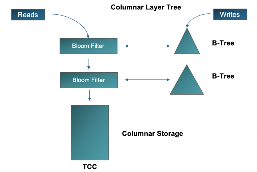
In this case, the B-Trees are ordered by the columnar record identifier so that we can merge the B-Trees with columnar data during reads.
The combination of Layer Trees, Bloom Filters, Top Class Containers changes the fundamental way for different systems – transactional and analytical – to be consistent. It solves a real problem, that the upper layers just can’t. It automatically solves the age-old “vacuuming” problem in typical columnar solutions and is at the same time, crash-safe. Consistency is always on, not eventual, yet accommodates the latency required to transform a row structure into a columnar structure. No more misdirects or euphemisms.
The “vacuuming” problem in typical Columnar solutions refers to heavy updating and inserting of data
fragments columnar structures (databases) making them un-performant, such that many organizations
have two columnar structures – as one gets slow, the other is put on line – sometimes referred to
as flip-flopping, causing all sorts of administrative headaches.
Sometimes it’s the little things that matter. Our reliance on the cloud ought to compel us all to think smarter and deeper rather than accept data being late, not available or untrustworthy. The plethora of databases may be one man’s index of creativity but if they do not come together, it’s a yard sale.
Ready to try Xpand in the cloud?