This is part 2 of a 5-part series, if you want to start from the beginning see Temporal Tables Part 1: Introduction & Use Case Example
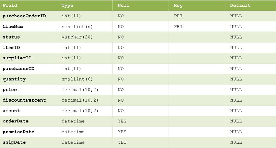
In part 1 of this blog series, we introduced a simplified purchaseOrderLines table:
and a series of operations that inserted and edited a record in the table:
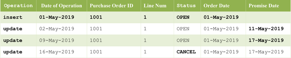
We now want to use MariaDB temporal features to ensure that we can retrieve the state of the record as of 02-May-2019, even though several updates have happened since 02-May-219 that have overwritten data.
System versioning is enabled via standard data definition language (DDL) syntax during table creation.
CREATE TABLE purchaseOrderLines(
    purchaseOrderID INTEGER NOT NULL
  , LineNum SMALLINT NOT NULL
  , status VARCHAR(20) NOT NULL
  , itemID INTEGER NOT NULL
  , supplierID INTEGER NOT NULL
  , purchaserID INTEGER NOT NULL
  , quantity SMALLINT NOT NULL
  , price DECIMAL (10,2) NOT NULL
  , discountPercent DECIMAL (10,2) NOT NULL
  , amount DECIMAL (10,2) NOT NULL
  , orderDate DATETIME
  , promiseDate DATETIME
  , shipDate DATETIME
  , PRIMARY KEY (purchaseOrderID, LineNum)
) WITH SYSTEM VERSIONING;
Or, system versioning can be added after table creation with a simple ALTER TABLE statement.
ALTER TABLE purchaseOrderLines ADD SYSTEM VERSIONING;
This is all that is required for MariaDB to begin transparently capturing copies of rows in the PurchaseOrderLines table as they are modified. Simple queries that wish to inspect the record as a specific point in time add an additional temporal clause to the query.
SELECT *
FROM purchaseOrderLines
  FOR SYSTEM_TIME AS OF TIMESTAMP '2019-05-02 23:59:59'
WHERE purchaseOrderId = 1001;
But what is really happening behind the scenes? MariaDB creates two invisible columns on the purchseOrderLines table, row_start and row_end.
SELECT
  purchaseOrderID
, lineNum
, row_start
, row_end
FROM purchaseOrderLines
  FOR SYSTEM_TIME ALL;
You can see these columns by explicitly including them in your select statement.

These new columns are of datetime date type which allows 6 decimal places of precision.
Pulling the history of changes to a specific purchase order line is now a matter of using the FOR SYSTEM_TIME ALL or FOR SYSTEM_TIME FROM syntax:
SELECT *
FROM purchaseOrderLines
  FOR SYSTEM_TIME ALL
WHERE purchaseOrderId = 1001;
SELECT *
FROM purchaseOrderLines
  FOR SYSTEM_TIME FROM ‘2019-05-01 00:00:00’ to ‘2019-05-31 23:59:59’
WHERE purchaseOrderId = 1001;
Remember that temporal tables and query semantics are a first-class part of the SQL standard. This means that you can combine them with views, aggregates, windowing functions and all of the richness of the SQL language. Perhaps you need to present a precise picture your purchase order data to a reporting tool that does not understand how to construct temporal queries? Simply create a view that presents the information to the tool of your choice.
Here is another example. Do you believe that a moving average of the number of event tickets sold is a meaningful metric? That can now be accomplished with a single query.
Let’s use the following table:
CREATE TABLE concertEvents (
    eventID     INT(11) NOT NULL
  , name        VARCHAR(128) NOT NULL
  , venue       VARCHAR(128) NOT NULL
  , perfDate    DATE NOT NULL
  , tksSold     INT(11) NOT NULL
) ENGINE=InnoDB DEFAULT CHARSET=latin1 WITH SYSTEM VERSIONING;
Populated with the following tuples:
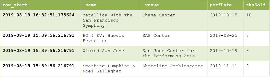
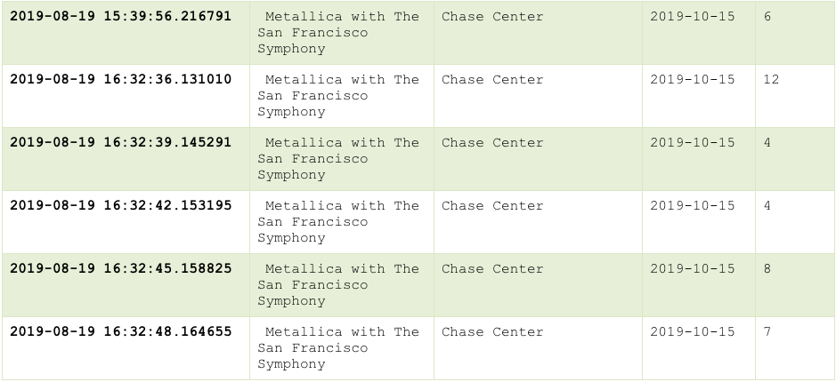
As you can see Metallica’s ticket count has been updated roughly every three seconds. We can obtain the moving average of tickets sold between a period of time as shown below:
SELECT
    e1.eventID
  , e1.name
  , ( SELECT
          SUM(tksSold) / COUNT(tksSold)
       FROM concertEvents
           FOR SYSTEM_TIME FROM '2019-08-19 15:39:56' TO '2019-08-19 16:32:51'
       WHERE eventID=e1.eventID ) AS 'Moving Avg'
FROM concertEvents AS e1
WHERE eventID = 1
GROUP BY e1.row_start;
This query shows the tickets sold moving average for the Metallica concert from ‘2019-08-19 15:39:56’ to ‘2019-08-19 16:32:51’.

Similarity, to retrieve the moving average for all the time
SELECT
    e1.eventID
  , e1.name
  , ( SELECT
          SUM(tksSold) / COUNT(tksSold)
      FROM concertEvents
          FOR SYSTEM_TIME ALL
      WHERE eventID=e1.eventID ) AS 'Moving Avg'
FROM concertEvents AS e1
WHERE eventID = 1
GROUP BY e1.row_start;
Will produce the following output:

Performant, native SQL access to temporal data opens up a whole range of possibilities. Because computations are performed in the database server, close to the data, the above types of queries can be much faster than equivalent implementations that are executed inside of Business Intelligence (BI) tools or custom code.
Continue to Temporal Tables Part 3: Managing History Data Growth to learn more.