How Xpand Works: Examining Distributed Continuation, Distributed Join and Distributed Aggregates

In internal measurements, MariaDB Xpand delivers very high price / performance.

These results are the consequence of the Xpand architecture and the key reasons include Distributed Continuation, Distributed Joins, and Distributed Aggregations:

1. Distributed Continuation¹

Modern software is increasingly Serverless.² Underneath creative pricing structures and auto-provisioning, Serverless technical architecture means that each unit of work is an autonomous task, severed from any permanently reserved resource.

Xpand takes this to the extreme. We call it Distributed Continuation. The units of work are called Fragments. Fragments are fully autonomous, and are down to the level of elemental operations on individual tuples of data. They execute bits of logic that run to completion, in accordance with the principles of the continuation-passing style of programming (CPS), and forward the continuation context to the next step as a one-way message (there is no call stack as with subroutines and no callbacks either). Physically, they are implemented as snippets of actual byte code.

Fragments are coroutines that process queries in parallel, each pinned to a core for the duration. They are generated by the Planner when it compiles the query and are distributed throughout the nodes of the Xpand cluster. Fragments operate on data tuples that are passed via a parallel Dataflow Execution Model³ whose transitions are solely one-way forwarding, with no round trips, no loops or cycles. Whatever “waiting” there is occurs only at “barrier-sync” points. Waits are implemented as yielding actions and so consume no resources, nor block or in any way affect operation of other fragments.

At the logical and architectural level there are no Primary and Secondary, no Leaders and Followers, and with a few peripheral exceptions⁴ – no centralized Coordinators of anything. There are no see-all / watch-over-all Resource Managers tasked with rationing things, no centralized Supervisors of anything. In fact – there is practically nothing besides Fragments and queues of Continuations – Serverless par excellence.

How it works, and what it does

As stated, the Xpand compiler generates Fragments that get dynamically installed and cached on all nodes of the cluster. You can think of them as a team of autonomous agents assembled for a purpose, each with its own skill set and responsibility, who jointly execute a business process.

Except that in our case, these agents work independently from each other, and they do not chat with each other, or wait on each other. Each takes a work order from an incoming queue, does what it is supposed to do, creates work orders for others, and pushes them into the others’ queues. Fire and quickly forget. Ultimately, the last agent in the sequence forwards the result back to the requesting user.

Xpand was built from the ground up for share-nothing clusters of machines. As is natural for such an architecture, it persists data in “slices”, which are spread among the nodes.⁵ Dataflow directs work orders to agents using the “function to data” (as opposed to “data to function”) principle. For example, a work order to fetch rows by a secondary index would be first directed to a node which holds the required index entry.⁶ Once the agent operating there retrieves the target row IDs, that agent creates work orders to fetch the desired rows and route them to the appropriate nodes. The agent is immediately ready to pick another work order, or go idle if there are none in the queue.

Agents are highly specialized,⁷ their work orders are extremely fine-grained (down to a single row or tuple), and are expected to complete their tasks very fast. This design allows them to operate without constant interruption, and so bypass all the overhead of context switching inherent in thread-based parallelism (or process-based). Instead, they are pinned to the cores and go into action every time a previous agent occupying this core completes, in the order determined by the queue of the work orders. They voluntarily yield when they run into a “blocking” operation like a latch or an I/O, or, in some exceptional cases of large and complex work orders, when a threshold of the allotted time is reached.

And so, how is this superior price / performance demonstrated by the benchmarks achieved?

Simple. The ecosystem of result-oriented agents is self-governed and does not depend on the top-down command-and-control “resource rationers”, “work supervisors”, and other central “governors”. Likewise, we avoid the overhead of the generic thread and process managers.

Share-nothingness, once properly exploited as opposed to fought against, allows us to eliminate practically all such waste.

The end result is an extremely high “Efficiency Ratio”, or, in the language of database systems, best possible price / performance, in our case approaching 1.

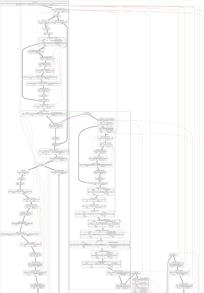
As an illustrative example, here is a slightly photoshopped portrait of two agents / fragments during work hours, working on

select * from table1 clx inner join table2 xp on clx.b = xp.b;

The red line indicates the place and time when the fragment on the left is passing the work order to the one on the right.

2. Distributed Join

It’s best to describe how we do distributed joins using simple examples. Let’s assume the following schema:

sql> CREATE TABLE bundler (
     id         INT      default NULL auto_increment,
     name       char(60) default NULL,
     PRIMARY KEY (id)
);

sql> CREATE TABLE donation (
     id         INT default NULL auto_increment,
     bundler_id INT,
     amount     DOUBLE,
     PRIMARY KEY (id),
     KEY bundler_key (bundler_id, amount)  
);

Here we have three indexes:

• _id_primary_bundler (primary key of bundler table)
• _id_primary_donation (primary key of donation)
• _bundler_key_donation (secondary index)

Note that in Xpand primary keys are what SQL Server calls “clustered indexes” (i.e. the data is kept with the index), while the secondary index only includes the Primary Key(s) of the matching rows.

Now, both _id_primary_bundler and _id_primary_donation are distributed based on the “id” fields. The _bundler_key_donation is distributed based on bundler_id, which may or may not be unique. Of course all rows with the same key value go to the same node.

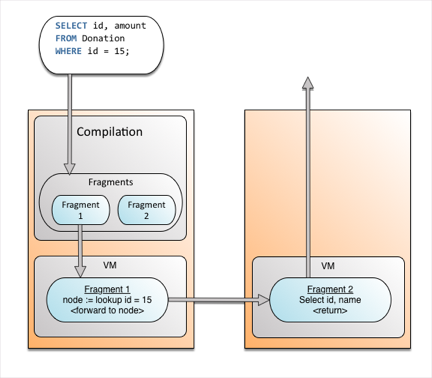
Let’s start with a trivial query:

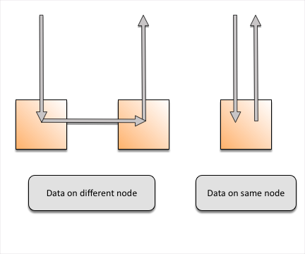
sql> SELECT id, amount FROM donation WHERE id = 15;

The data will be read from one of the replicas.⁸ This can either reside on the same node or require one hop. The diagram below shows both cases. As the dataset size and the number of nodes increase, the number of hops that one query requires (0 or 1) does not change.⁹ This underpins the linear scalability of point reads and writes.

Workflow

Physical Implementation

Now let’s look at joins. Key elements of the architecture are:

• Tables and indexes have their own independent distribution. Therefore we are always able to determine which node/replica to go to on nested loops, without having to resort to broadcasts.
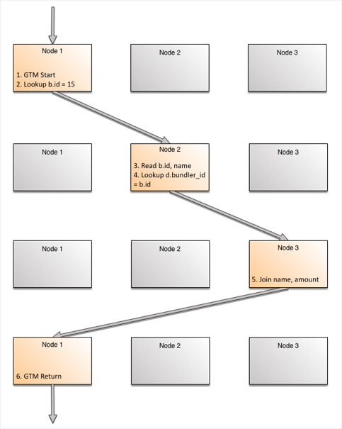
• There is no central node orchestrating data motion, and running request-response protocols. Data moves to the node needing it next. Let’s look at a query that gets the name and amount for all donations collected by the particular bundler, known by id = 15.

sql> SELECT name, amount from bundler b 
JOIN donation d on b.id = d.bundler_id WHERE b.id = 15;

The query optimizer will look at the usual statistics like distributions, hot lists, etc. to determine a plan:

1. Start on the node which receives the query
2. Lookup node/replica which contain the required row  _id_primary_bundler has (b.id = 15) and forward a work order to that node
3. Read b.id, name from the  _id_primary_bundler
4. Lookup nodes/replicas which contain _bundler_key_donation (d.bundler_id = b.id = 15) and forward the order to that node
5. Join the rows and forward to originating node
6. Return results to the user.

The key here is in step #4. For joins, when the first row is read, there is a specific value for the foreign key. The target node can be identified precisely.

Let’s see this graphically. Each returned row has gone through the maximum of three hops inside the system. As the number of returned rows increases, the work per row does not. Rows being processed across nodes and rows on the same node running different fragments use concurrent parallelism by using multiple cores. The rows on the same node and same fragment use pipeline parallelism between them.

Now let’s drop the unique predicate b.id=15. The join will now follow the scan, and like the scan will run in parallel on multiple machines.

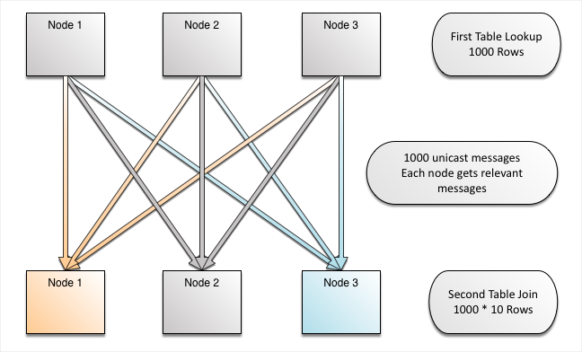
But, what’s important here is that each node is only getting work orders for the rows that actually reside there,¹⁰ again delivering the highest possible efficiency ratio.

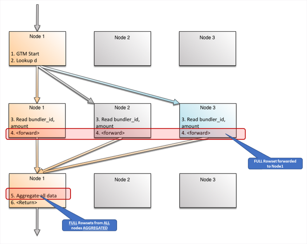
3. Distributed Aggregates

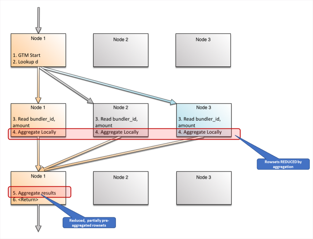
In Xpand, partial aggregations run in parallel on multiple nodes, and within each, on multiple cores. Typically, the degree of parallelism for an individual query inside each node would be proportional to the number of slices needed by the query which reside on that node.

Let’s say we have a query that aggregates the data over an entire table.

sql> SELECT id, SUM(amount) FROM donation d GROUP BY by bundler_id;

The nodes will mobilize the expert agent specializing in partial aggregation roughly one for each slice, in order to achieve the independence of the data scan. This will naturally reduce the volumes of data which would need to be merged in order to complete the job.¹¹

There are also variants of merge – aggregate logic. For example, if the GROUP BY happened on an indexed column, the partial aggregates will be streamed in the order of that column, offering the opportunity to optimize the final aggregation algorithm (manifested as a so-called “streaming aggregate”, as opposed to “partial aggregate” in other cases ).

And in some cases this can go further:

sql> SELECT DISTINCT bundler_id FROM donation;

Remembering that bundler_id is an index, we know that (i) its values on each node are unique to this node and do not repeat elsewhere, and (ii) they are, within each node, sorted. This allows us to reduce partial aggregation with mere deduplication, and also to reduce the final merge to simply merge the incoming streams blindly and at practically no cost.

Roads not taken

A very effective method of describing things is to define them by their opposite, by what they are not.¹²

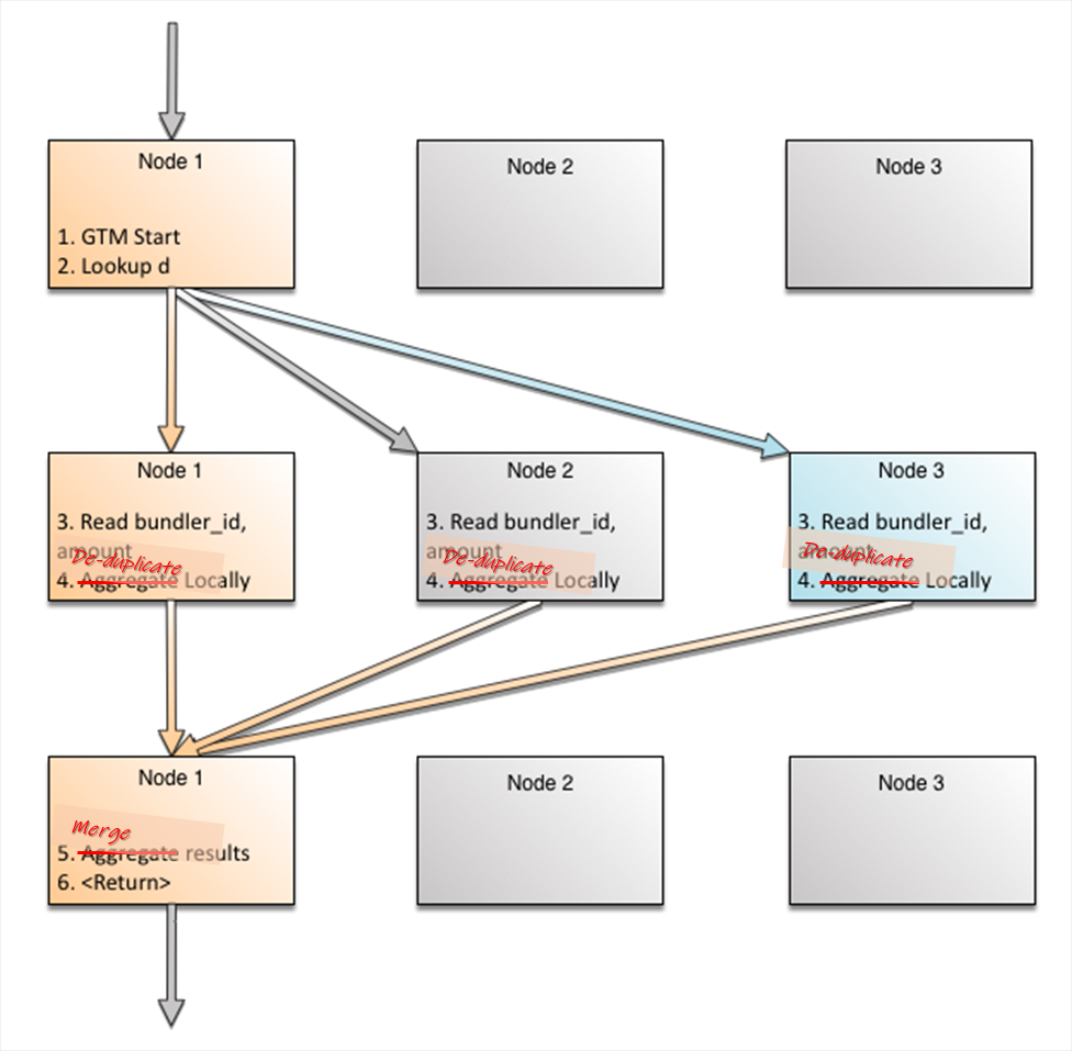
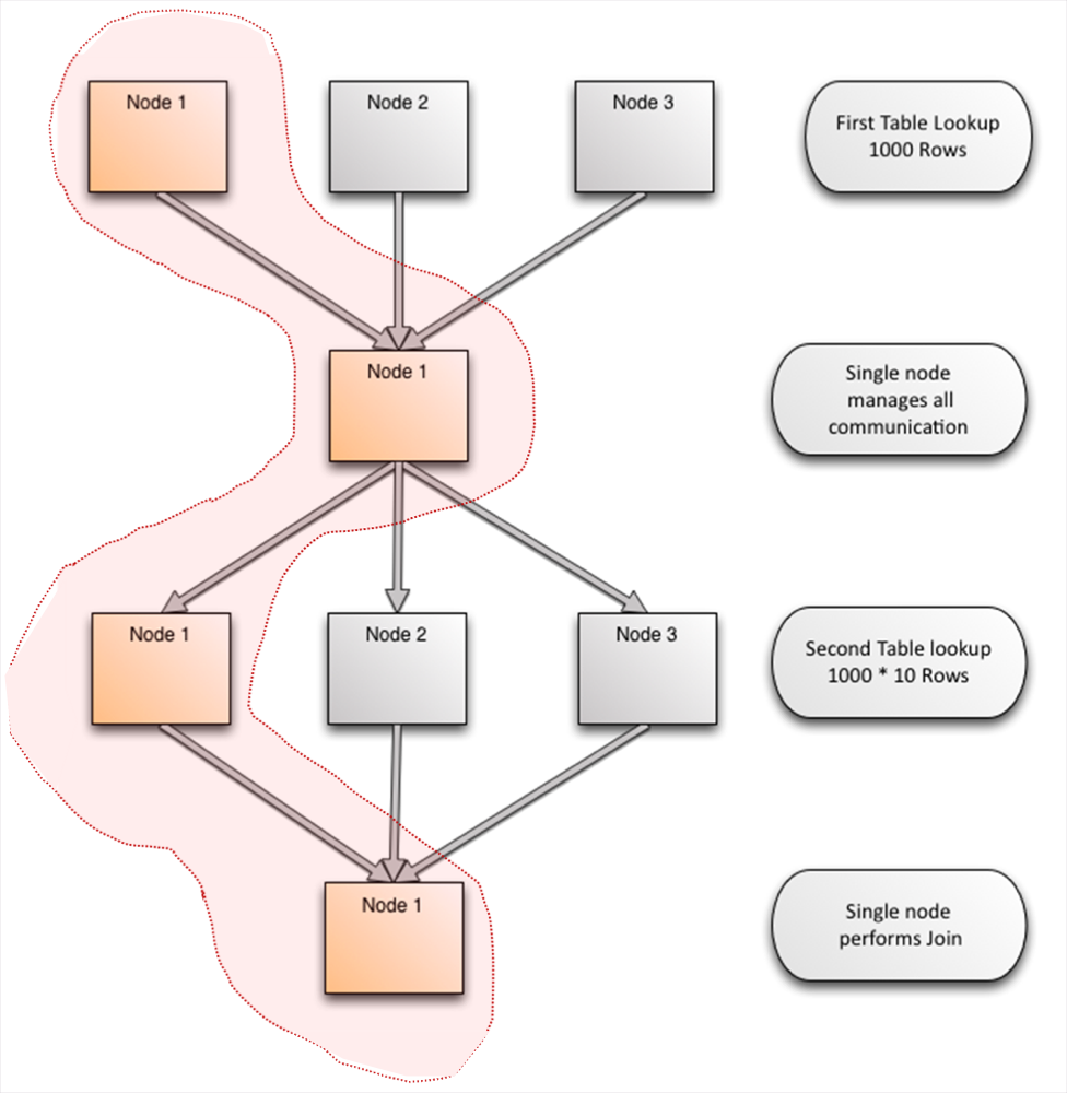
The Curse of a Master Node

Intellectual traps, if one falls in them, have consequences. For solutions that rely on a Master node, all joins and aggregations happen on the single node that is handling the query. This ends up moving a lot more data, and is unable to use the resources of more than one machine.

Joins

Aggregates

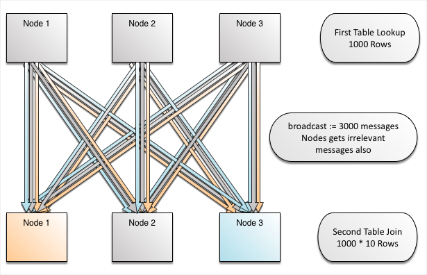
The Temptation of Co-Locating Rows and Secondary Indexes

One of the common intellectual traps vexing designers of distributed systems is how to deal with secondary indexes. It is tempting to  distribute indexes according to the primary key and so achieve a supposed “co-location”, which intuitively suggests that this would yield a smaller number of node hops in some cases. This, however, creates a significant problem for distributed architectures.

Given an index on a column like bundler_id in the previous example, the system has no clue where that key goes, since distribution was done based on donation.id. This leads to broadcasts, and, worse yet, to broadcast overheads, i.e. communications with the nodes, which in a large proportion of cases will have no matching data.

Recap

The MariaDB Xpand architecture can be summarized as a highly efficient implementation of serverless computing, producing a scale-out parallel autonomous execution engine.

While application developers may not need to know the internals of this architecture, it is important that they can now rely on a familiar and accessible database substrate that can be elastically sized based on need, including the highest levels in price-performance, as well as resilience and dependability.

As one of the few distributed databases built from the ground up, with production implementations across the world, we believe we have created a simpler yet more powerful database paradigm that improves the viability and success of forward thinking applications. We have also broken new ground in the very nature of how databases are imagined and engineered.

Get started with MariaDB Xpand today.

Footnotes

¹https://en.wikipedia.org/wiki/Continuation-passing_style
https://en.wikipedia.org/wiki/Continuation

²https://en.wikipedia.org/wiki/Serverless_computing

³https://en.wikipedia.org/wiki/Dataflow_programming
https://en.wikipedia.org/wiki/Dataflow_architecture

⁴ There is a coordinator for cross-cluster parallel asynchronous replications running on the receiving end of it charged with declaring that there is time to commit the accumulated bulk.

⁵ This of course requires good and equitable distribution of slices between the nodes. Xpand includes a unique component called Rebalancer, which monitors the skewness of slices, and takes corrective actions to keep it in constant balance, while running in the background. Additionally, there is a configurable layer of redundancy to support HA (High Availability)

⁶Xpand distributes secondary indexes independently from the rows. The benefits of this design will be seen in later chapters.

⁷Each agent’s specialized task may be thought of as a particular step in a query plan.

⁸There is an elaborate scheme by which the Balancer picks up and designates one specific replica as “ranking”, in order to balance read traffic
among the nodes more effectively.

⁹Of course if there are two or more replicas, there will be at least one hop for writes (since both replicas cannot reside on the same node).

¹⁰The colors on the receiving nodes match those on the arrows – this is to indicate that rows are flowing correctly to nodes where they will find matching data for successful join.

¹¹This classic technique is nowadays called “map-reduce”, and is portrayed as a significant innovation in computer science. At some point prior it was called “scatter-gather”. Earlier still it was not called anything at all and was considered self-evident thus requiring no special designation.

¹² The method bears the name “Apophatic,” from ancient Greek ἀπόφημι – pronounced as apophēmi, meaning “to deny.”